I’ve written this post to accompany the talk I gave on August 31 to the UW Cartography Lab’s Education Series special two-day workshop in partnership with Mapbox. I was asked to talk about JavaScript and Turf.js. Give my mixed audience, I thought talking about Turf right away would be putting the cart a bit before the horse—first, I needed to build a simple web GIS app that could use Turf. So this 1-hour talk turned into an as-noob-friendly-as-possible walkthrough of building such an app.
To start, here are the slides I used; really, just an outline of my talk.
The link on the second slide goes to a dropboxed zip file containing two directories: one called “initial” and another called “final.” The “initial” directory contains a boilerplate HTML file that I used to begin my live app-building demo and a data directory with two zip files. The “final” directory contains the final app script and data files. I’ll be walking through the “final” version, but you can start with “initial” and try to build it out yourself for practice.
Slide 3 is what I called the “Sam Matthews Mantra.” Sam Matthews is this awesome guy who I used to work side-by-side with in the Cart Lab back in 2012 and now works at Mapbox; his visit to Madison was the original impetus for this “reunion” event. Yesterday, he gave a talk on the basic structure of slippy maps, including the four ingredients: tiles, library, data, and internet. But for the purposes of my tutorial, I modified this mantra a bit (slide 4) to outline the parts of my demo: library, tiles, data, and analysis.
To create my app, I first needed to load some helper libraries. The app uses jQuery to interface with the DOM (Document Object Model, the structure of a website) and facilitate asynchronous communication between the browser and server. For the actual mapping, I used Leaflet, now the most popular open-source JavaScript library for creating web maps. The spatial analysis components that make this a web GIS app uses Turf.js, but I’ll get into that library more later. I call the libraries from remotely hosted sources using some simple script tags in the <body> section of index.html:

Leaflet also requires its own stylesheet, linked in the header:

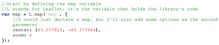
With Leaflet imported, we can build a basic map with the following JavaScript code within the $(document).ready callback function (this bit of jQuery causes the browser to wait until the entire page is loaded before executing the JavaScript):
Awesome—I now have a Leaflet map; you can tell by the zoom button in the upper-left corner. Note that I am running the app through a Localhost server, rather than double-clicking on the index.html file. Some browsers (Chrome especially) strongly dislike loading data outside of a server, so it’s always best to set one up first. If you don’t want to go through the rigmarole to set up something permanent on your machine, a great temporary solution is to run your app through a preprocessor app such as prepros or codekit.
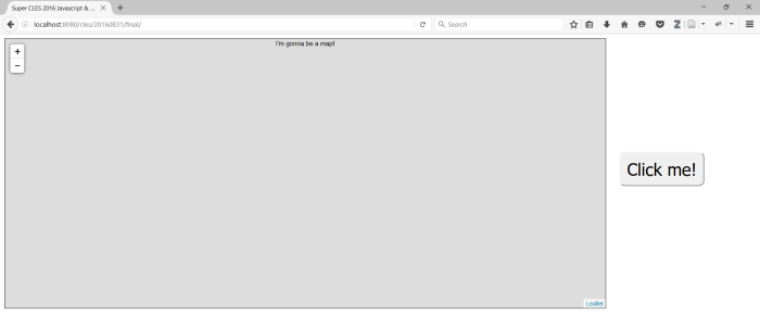
(The text and “Click me!” button were included in the “initial.html” template).
It’s not really much of a slippy map, though, without some map tiles. Nowadays, I like to choose tilesets for my Leaflet apps that are included in the Leaflet Providers Preview. Leaflet-providers is a small plug-in for Leaflet that lets you use a shorthand tileset name instead of a full tileset URL to create a Leaflet tile layer, but the Preview site is itself a handy tool that gives you the full code for creating the tile layer if you don’t want to download the plug-in. For my purposes in this demo, I just copied and pasted the code for the Stamen Watercolor tileset:
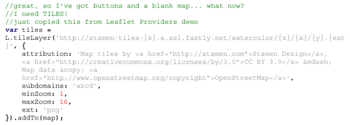
A little explanation of the above: L.tileLayer is a method of Leaflet that creates a tile layer. It takes two parameters: a URL with variables (letters inside curly braces) that are replaced by the library automatically depending on which tiles are called from the server, and an options object with any of several options for the tile layer. The addTo method then adds the new tile layer to the Leaflet map object, contained by the map variable.
With tiles loading, it’s time for data! For the demo, I chose to use two datasets from Natural Earth, the go-to website for popular global datasets covering cultural, physical/natural, and raster themes. The two datasets I chose were States and Provinces and Populated Places, both at the 1:50 million (medium) scale (unbeknownst to either of us before hand, John Czaplewski, who presented after me, chose the exact same datasets for his live PostGIS demo). To prevent any snafus with the Natural Earth site (it was being slow when I tested it the night before), I went ahead and included these two shapefiles in the “initial” demo folder, each in its own zip archive (“states.zip” and “places.zip”).
If you’ve ever worked with GIS software, you probably know what a shapefile is. Really, it’s a collection of several different files with different components of a geospatial dataset (the .shp component contains the geometry data, while other components contain attribute data, metadata, etc.). Shapefiles are a popular standard format for GIS data (though not usually the best one for spatial analysis tasks), but they’re pretty useless for web apps. Instead, the standard geospatial data format for the web has become the GeoJSON format.
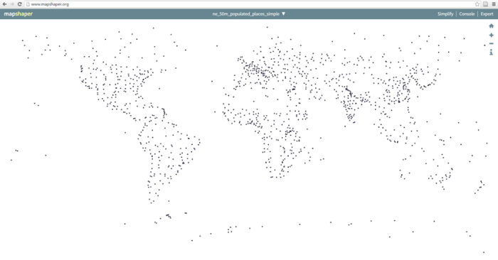
A handy tool for converting shapefiles to GeoJSONs is mapshaper, created by UW alumnus and New York Times graphics wiz Matt Bloch. We can import a shapefile to mapshaper by just dragging the .shp part of the file and dropping it on the site, but that will result in only the geometries being converted to GeoJSON without any attributes. We want the attributes, so we need the whole shapefile; luckily, mapshaper lets us import a zip file containing it. Once we’ve uploaded a shapefile, mapshaper should display something like this:
Mapshaper is a great little program. It allows you to quickly and easily simplify polygon geometries, reducing the file size. In this case, though, all we want it to do is spit the data back out as a GeoJSON. For this, we click on “Export” in the upper-right corner, then choose “GeoJSON” and hit “Export” again. This should cause a .json file to download. To make accessing the data easier, I renamed each file “places.geojson” and “states.geojson,” respectively.
Now, just what is a GeoJSON? It’s a geospatial variant of JSON, which stands for “JavaScript Object Notation.” Essentially, it’s a more picky formatting of a JavaScript “object,” which is really not an object in the true object-oriented programming sense but rather a type of map or dictionary data container. To see what this looks like, neatly formatted, we can import our new GeoJSON data into another handy little web app called geojson.io, an open-source project largely created by Mapbox’s Tom MacWright. Here is our populated places file displayed in it:
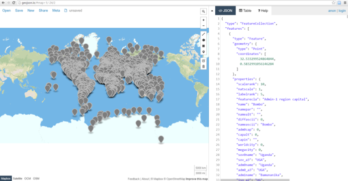
On the right-hand side of the window, you can see the object structure of the file, which consists of nested key-value pairs. Every GeoJSON has a "type" which is always "FeatureCollection", and every one always has a "features" property consisting of an array of features. This will become important when we use Turf.js to operate on the data. Each feature in turn has a "type", which is always "feature", a "geometry" which is an object containing the feature geometry as one or more geographic coordinate pairs (always in the WGS 84 coordinate system), and a "properties" object consisting of the attributes, if any. Note that this is similar to a shapefile in that it doesn’t encode any relationships between features, or topology in GIS speak (there is another web spatial data format, TopoJSON, which does encode topology, but we won’t get into that in this tutorial).
Now that we have our data in the right format, we need to load it into our code and onto the map. Loading data into a JavaScript program is trickier than it sounds, but it’s worth taking the time to show you how to do it right. Some tutorials out there will tell you to just assign a variable to the code in each JSON file and bring it into the site with HTML <script> tags, but if you’re loading geographic datasets (which tend to be large), this has a tendency to bog down the loading of your page. It’s much better to load the data asynchronously, adding it to the page after it has loaded into the script. But this means that the rest of your script will have executed before your data is loaded. Thus, you need a special function called an AJAX callback to make use of your data only after it has been loaded by the browser.
First, we need to make sure our .geojson files are stored in the “data” folder of our working directory. Then, we can use one of jQuery’s many helpful AJAX methods to load the data into our script. Because we have two datasets we need to load, it’s best to load them in parallel (at the same time) and only call the function that uses the data (the callback) after both files have loaded. To do this with jQuery, we can use the $.when method:
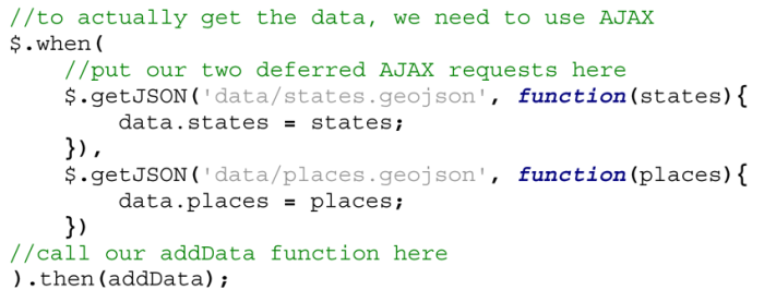
Note that the two $.getJSON methods are actually parameters of the $.when method, so there should be a comma between them, and no semicolons in between or after them (I ran into trouble with this both in practicing for the demo and doing it). Each one of these .getJSON methods calls a data file and then executes a separate callback for that file, which saves the file’s data to a property of an object I created previously (data). Finally, the .then method calls the overall callback function after the data has loaded, which I’ve named addData. Now, I’ve put a few carts before the horse here; let’s back up and take a look and where I define the data object and the addData function, above the AJAX call:
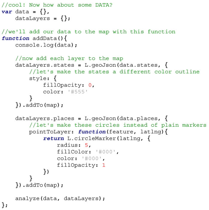
Again, this code is above the $.when method in the script. Here, I’m first defining two objects: data, which (as we have already seen) will hold the GeoJSON data, and dataLayers, which will hold Leaflet’s rendering of that data into layer objects that can go on our map.
Then I define the callback function, addData. By the time this function executes, the $.getJSON callbacks have already saved each file’s GeoJSON data to properties of the data object, so I can go ahead and take a look at the structure of that object in the console and see that my data is indeed present:

Now that I have this data, I can use Leaflet’s L.geoJson method to stick each layer on the map. This method takes two parameters: the data I want to turn into a map layer, and an options object that can hold a number of different layer options. For the states layer, I’ve given it some style options to override Leaflet’s defaults. For the places layer, I’m using the pointToLayer option to create a function that iterates over each point feature and turns it into a Leaflet circleMarker, which I have styled to look like a moderately-sized black dot. Each L.geoJson method is chained to the .addTo(map) method to add it to the map, and the resulting layer object is assigned to a property of the dataLayers object I created above the addData function, allowing for later access.
Here is what my map now looks like:

With data on the map, we are ready for the fourth and final step, which makes this a true WebGIS: analysis. Now, as you can see in my HTML and the image above, I have included a large “Click me!” button in the boilerplate for the app. A good WebGIS should be interactive; you want to allow your users to perform operations on the data, not just do what you think they want to do for them. Since this is a simplified demo, I figured I would just include one button instead of several to demonstrate the concept. At the end of the tutorial, each click of the button will do something different and interesting to the data.
Before we get there, to keep our code neat and make sure the analysis only gets performed after the data is loaded, we need a new function called from within addData to put our analysis tasks in. I’ve called this function analyze, and pass it the two objects I created, data and dataLayers. If you’re working from the “initial” index.html file, you will want to move the $('#mybutton').click listener and clickme callback function inside of this analyze function. Inside analyze, we will perform three types of analysis using Turf.js: a point-in-polygon test, creation of a bounding box, and creation of a triangulated irregular network (TIN). To have our button do each of these in turn, we will create a counter and increment it each time the button is clicked, calling a different analysis function for each counter value.
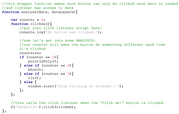
Before we go further, the thing to know about Turf is that its methods operate very much like toolboxes in ArcGIS: you put one or more layers in and you get a new layer out. The big difference is that in this case, each layer is in GeoJSON format, either an individual feature or an entire FeatureCollection. Turf includes dozens of helpful analysis tools that can all be run client-side in the browser. This gets an A+ for convenience and interactivity, but a C or D for performance. If you’re using big data or have a complex series of tasks to run, fire up Arc or Q or Python and skip the JavaScript.
Now, let’s create our point-in-polygon function. A point-in-polygon test is a classic problem in computational geometry and has all sorts of applications in GIS. Turf’s .within method accomplishes this test. It takes two parameters—a set of points and a set of polygons—and returns a new FeatureCollection containing just the points that are within the polygons. So, say we want to find the populated places within the U.S. lower 48 states. Since our states dataset has states and provinces for other countries as well, we will first have to pick out only U.S. states that aren’t Alaska or Hawaii and add them to the features array of a new FeatureCollection. We can do this with a piece of native JavaScript, a .forEach loop:

Now that we have our subset of states—stored in the usStates variable—we can use it to perform our point-in-polygon test, and view the results in the console:
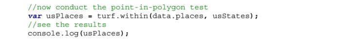

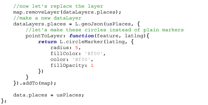
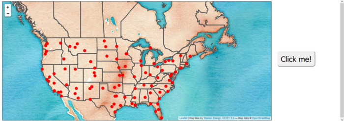
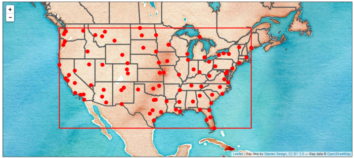
There are 94 populated places within the U.S. Lower 48 out of our original dataset. To put these on the map, we can simply create a new L.geoJson layer (this time with red dots) and add it to the map. We can also replace the places component of our data object with the new dataset, so that our next two analysis operations are only operating on the U.S. places.
Now when we click on the “Click me!” button, we should see this result:
That was actually the hardest Turf analysis I got to in the demo. I wanted to get the tough one out of the way first, I guess. The next two are much more simple. First, the bounding box:
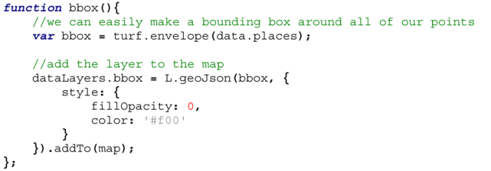
This uses Turf’s .envelope method to return a polygon encompassing all vertices. Once again, it makes a call to L.geoJson to plunk the bounding box onto the map. Voilá:
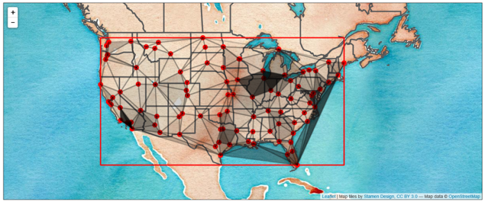
Finally, we’ll create a TIN using our U.S. Places as the input dataset. Turf’s .tin method takes the dataset and optionally the name of an attribute that can be used as a z value for each vertex. This results in polygons that have three properties: a, b, and c, the z values. We can use this data to shade the triangles; in this case, I chose to calculate the averages of the three values and use each polygon’s average to derive its percentage of the highest average z value in the dataset. I then set this percentage as the opacity of the polygon to make the data visible.

Here is the result (after three button clicks):
That’s about it for this demo. Of course, there are lots of ways to use Turf that don’t involve Leaflet; since it speaks GeoJSON, it’s compatible with a wide variety of other libraries and frameworks. Hopefully this has been a useful intro to open source WebGIS tools and inspires you to go do something cool.
